Note
Go to the end to download the full example code.
06. Analyze SEF Data with OPM#
This example demonstrates how to analyze somatosensory evoked field (SEF) data collected with optically pumped magnetometers (OPM) and compare it with superconducting quantum interference device (SQUID) data. The OPM data was obtained with the background field nulling coils we developed.
# Author: Mainak Jas <mjas@mgh.harvard.edu>

import json
import matplotlib.pyplot as plt

import mne
from opmcoils.analysis import find_events, add_ch_loc, read_opm_info

from pathlib import Path
import pooch

# sphinx_gallery_thumbnail_number = 3
First, use pooch to download the data
url = "https://osf.io/aqh27/download"

target_dir = Path.cwd() / 'data'
project_dir = target_dir / 'sef_data'

path = pooch.retrieve(
    url=url,
    known_hash=None,  # We don't know the hash
    path=target_dir,
    fname='sub-01.zip',  # Specify the filename
    processor=pooch.Unzip(extract_dir=project_dir),  # Extract to a folder named 'sub-01'
    progressbar=True
)
Then, we define the file paths
subject = 'sub-01'
date = '20240722'
cond = 'median'

subjects_dir = project_dir / subject
raw_fname = subjects_dir / 'opm_meg' / date / f'{date}_{subject}_paneltesting_{cond}_raw.fif'
raw_fname_squid = subjects_dir / 'squid_meg' / date / 'RT_median_raw.fif'
helmet_info_fname = target_dir / 'helmet_99channel_size-60.fif'
ch_mapping_fname = subjects_dir / 'opm_meg' / date / 'mapping.json'
Then, we start by processing OPM data
bads = ['01:15', '00:14', '00:15', '00:16']

raw_opm = mne.io.read_raw_fif(raw_fname, preload=True)
raw_opm.rename_channels(lambda x: x.strip('-BZ_CL'))
raw_opm.info['bads'] = bads

raw_opm.set_channel_types({'Input-1': 'stim'})
Opening raw data file /Users/mainak/Desktop/04_github_repos/opm_coils/examples/data/sef_data/sub-01/opm_meg/20240722/20240722_sub-01_paneltesting_median_raw.fif...
Isotrak not found
    Range : 0 ... 303721 =      0.000 ...   303.721 secs
Ready.
Reading 0 ... 303721  =      0.000 ...   303.721 secs...
Electrical median nerve stimulation creates artifacts. We will annotate the artifacts to avoid filtering the sharp transients.
events = find_events(raw_opm, min_duration=1. / raw_opm.info['sfreq'])
annot = mne.annotations_from_events(events, raw_opm.info['sfreq'],
                                    event_desc={1: 'BAD_STIM'})
# XXX: annotations_from_events should have duration option
annot.onset -= 0.002
annot.duration += 0.003

raw_opm.notch_filter(60.)

raw_opm.set_annotations(annot)
raw_opm.filter(4., None, skip_by_annotation=())
raw_opm.filter(None, 150, skip_by_annotation=('BAD_STIM'))
608 events found on stim channel Input-1
Event IDs: [1]
Filtering raw data in 1 contiguous segment
Setting up band-stop filter from 59 - 61 Hz

FIR filter parameters
---------------------
Designing a one-pass, zero-phase, non-causal bandstop filter:
- Windowed time-domain design (firwin) method
- Hamming window with 0.0194 passband ripple and 53 dB stopband attenuation
- Lower passband edge: 59.35
- Lower transition bandwidth: 0.50 Hz (-6 dB cutoff frequency: 59.10 Hz)
- Upper passband edge: 60.65 Hz
- Upper transition bandwidth: 0.50 Hz (-6 dB cutoff frequency: 60.90 Hz)
- Filter length: 6601 samples (6.601 s)

Filtering raw data in 1 contiguous segment
Setting up high-pass filter at 4 Hz

FIR filter parameters
---------------------
Designing a one-pass, zero-phase, non-causal highpass filter:
- Windowed time-domain design (firwin) method
- Hamming window with 0.0194 passband ripple and 53 dB stopband attenuation
- Lower passband edge: 4.00
- Lower transition bandwidth: 2.00 Hz (-6 dB cutoff frequency: 3.00 Hz)
- Filter length: 1651 samples (1.651 s)

Filtering raw data in 609 contiguous segments
Setting up low-pass filter at 1.5e+02 Hz

FIR filter parameters
---------------------
Designing a one-pass, zero-phase, non-causal lowpass filter:
- Windowed time-domain design (firwin) method
- Hamming window with 0.0194 passband ripple and 53 dB stopband attenuation
- Upper passband edge: 150.00 Hz
- Upper transition bandwidth: 37.50 Hz (-6 dB cutoff frequency: 168.75 Hz)
- Filter length: 89 samples (0.089 s)
Then, we create evoked response
reject = None # dict(mag=11e-12)
epochs_opm = mne.Epochs(raw_opm, events, tmax=0.3,  # ISI = 300 ms
                        reject_by_annotation=False,
                        reject=reject, reject_tmin=0.03,
                        preload=True)
evoked_opm = epochs_opm.average()
Not setting metadata
608 matching events found
Setting baseline interval to [-0.2, 0.0] s
Applying baseline correction (mode: mean)
0 projection items activated
Using data from preloaded Raw for 608 events and 501 original time points ...
1 bad epochs dropped
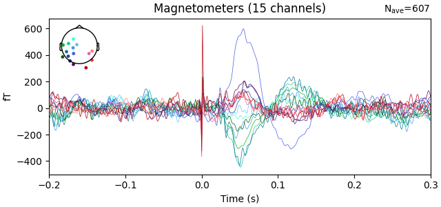
We add channel locations for the OPM sensors and plot the evoked response with spatial colors.
info_helmet = read_opm_info(helmet_info_fname)

with open(ch_mapping_fname, 'r') as fd:
    ch_mapping = json.load(fd)

add_ch_loc(evoked_opm, info_helmet, ch_mapping)

evoked_opm.plot()
Isotrak not found

<Figure size 640x300 with 2 Axes>
We use HFC to remove background artifacts.
projs_hfc = mne.preprocessing.compute_proj_hfc(evoked_opm.info, order=1)
evoked_opm.add_proj(projs_hfc)
evoked_opm.apply_proj()

# Alternatively, one could use SSP:
# projs_ssp = mne.compute_proj_epochs(epochs_opm.copy().crop(tmax=0), n_mag=2)
# evoked_opm.add_proj(projs_ssp)
# evoked_opm.apply_proj()
3 projection items deactivated
Created an SSP operator (subspace dimension = 3)
3 projection items activated
SSP projectors applied...
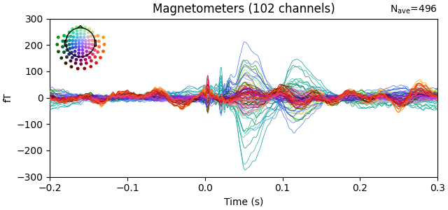
Let us now process the SQUID data.
raw_squid = mne.io.read_raw_fif(raw_fname_squid, raw_fname_squid, preload=True)
raw_squid.pick_types(meg='mag', stim=True)
events = mne.find_events(raw_squid, min_duration=1. / raw_opm.info['sfreq'])

annot = mne.annotations_from_events(events, raw_squid.info['sfreq'],
                                    event_desc={1: 'BAD_STIM'})
# XXX: annotations_from_events should have duration option
annot.onset -= 0.002
annot.duration += 0.003
raw_squid.set_annotations(annot)

raw_squid.filter(4., None)
raw_squid.notch_filter(60.)
raw_squid.filter(None, 150, skip_by_annotation=('BAD_STIM'))
epochs = mne.Epochs(raw_squid, events, tmax=0.3,
                    reject_by_annotation=False)
evoked_squid = epochs.average()
evoked_squid.plot(ylim=dict(mag=(-300, 300)))
Opening raw data file /Users/mainak/Desktop/04_github_repos/opm_coils/examples/data/sef_data/sub-01/squid_meg/20240722/RT_median_raw.fif...
    Read a total of 6 projection items:
        generated with dossp-2.1 (1 x 306)  idle
        generated with dossp-2.1 (1 x 306)  idle
        generated with dossp-2.1 (1 x 306)  idle
        generated with dossp-2.1 (1 x 306)  idle
        generated with dossp-2.1 (1 x 306)  idle
        generated with dossp-2.1 (1 x 306)  idle
    Range : 45000 ... 543999 =     22.500 ...   272.000 secs
Ready.
Reading 0 ... 498999  =      0.000 ...   249.500 secs...
NOTE: pick_types() is a legacy function. New code should use inst.pick(...).
496 events found on stim channel STI101
Event IDs: [1]
/Users/mainak/Desktop/04_github_repos/opm_coils/examples/plot_compare_sef.py:124: RuntimeWarning: Omitted 45 annotation(s) that were outside data range.
  raw_squid.set_annotations(annot)
Filtering raw data in 1 contiguous segment
Setting up high-pass filter at 4 Hz

FIR filter parameters
---------------------
Designing a one-pass, zero-phase, non-causal highpass filter:
- Windowed time-domain design (firwin) method
- Hamming window with 0.0194 passband ripple and 53 dB stopband attenuation
- Lower passband edge: 4.00
- Lower transition bandwidth: 2.00 Hz (-6 dB cutoff frequency: 3.00 Hz)
- Filter length: 3301 samples (1.651 s)

Filtering raw data in 1 contiguous segment
Setting up band-stop filter from 59 - 61 Hz

FIR filter parameters
---------------------
Designing a one-pass, zero-phase, non-causal bandstop filter:
- Windowed time-domain design (firwin) method
- Hamming window with 0.0194 passband ripple and 53 dB stopband attenuation
- Lower passband edge: 59.35
- Lower transition bandwidth: 0.50 Hz (-6 dB cutoff frequency: 59.10 Hz)
- Upper passband edge: 60.65 Hz
- Upper transition bandwidth: 0.50 Hz (-6 dB cutoff frequency: 60.90 Hz)
- Filter length: 13201 samples (6.601 s)

Filtering raw data in 452 contiguous segments
Setting up low-pass filter at 1.5e+02 Hz

FIR filter parameters
---------------------
Designing a one-pass, zero-phase, non-causal lowpass filter:
- Windowed time-domain design (firwin) method
- Hamming window with 0.0194 passband ripple and 53 dB stopband attenuation
- Upper passband edge: 150.00 Hz
- Upper transition bandwidth: 37.50 Hz (-6 dB cutoff frequency: 168.75 Hz)
- Filter length: 177 samples (0.088 s)

Not setting metadata
496 matching events found
Setting baseline interval to [-0.2, 0.0] s
Applying baseline correction (mode: mean)
Created an SSP operator (subspace dimension = 4)
6 projection items activated

<Figure size 640x300 with 2 Axes>
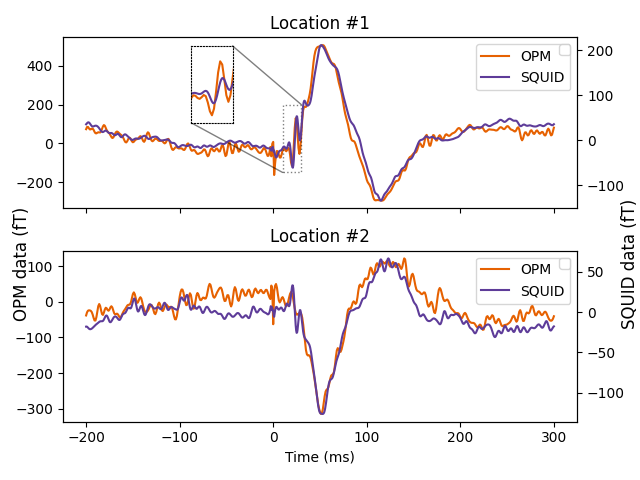
“Butterfly plots” are not appropriate to compare the evoked responses between OPMs and SQUID because the sensor locations are not comparable and hide individual sensor time series.
That is why, we pick sensors in similar locations on the OPM-MEG and SQUID-MEG and compare the evoked responses.
squid_chs = ['MEG0431', 'MEG0311']
opm_chs = ['MEG30', 'MEG09']
scale = 1e15
fig, axes = plt.subplots(2, 1, sharex=True)

for i, (opm_ch, squid_ch) in enumerate(zip(opm_chs, squid_chs)):
    ax = axes[i].twinx()
    ln1 = axes[i].plot(evoked_opm.times * 1e3,
                       evoked_opm.copy().pick([opm_ch]).data[0] * scale,
                       '#e66101')
    ln2 = ax.plot(evoked_squid.times * 1e3,
                  evoked_squid.copy().pick([squid_ch]).data[0] * scale,
                  '#5e3c99')
    axes[i].set_title(f'Location #{i + 1}')
    axes[i].legend(ln1 + ln2, ['OPM', 'SQUID'], loc=1)
    ax.legend()

fig.text(0.97, 0.45, 'SQUID data (fT)', va='center',
         rotation='vertical', fontsize=12)
fig.text(0.02, 0.45, 'OPM data (fT)', va='center',
         rotation='vertical', fontsize=12)
axes[1].set_xlabel('Time (ms)')
plt.tight_layout()
plt.show()

# Add inset
squid_ch, opm_ch = squid_chs[0], opm_chs[0]
inset_ax = axes[0].inset_axes([0.25, 0.5, 0.08, 0.45],
                              xlim=(10, 30), ylim=(-150, 200),
                              xticks=[], yticks=[])
inset_ax.plot(evoked_opm.times * 1e3,
              evoked_opm.copy().pick([opm_ch]).data[0] * scale,
              '#e66101')
inset_ax.plot(evoked_squid.times * 1e3,
              evoked_squid.copy().pick([squid_ch]).data[0] * scale,
              '#5e3c99')
for spine in inset_ax.spines.values():
    spine.set_linestyle('dotted')
axes[0].indicate_inset_zoom(inset_ax, edgecolor='black', linestyle='dotted')
/Users/mainak/Desktop/04_github_repos/opm_coils/examples/plot_compare_sef.py:156: UserWarning: No artists with labels found to put in legend.  Note that artists whose label start with an underscore are ignored when legend() is called with no argument.
  ax.legend()

(<matplotlib.patches.Rectangle object at 0x1af679bb0>, (<matplotlib.patches.ConnectionPatch object at 0x1af679d90>, <matplotlib.patches.ConnectionPatch object at 0x1af6a6130>, <matplotlib.patches.ConnectionPatch object at 0x1af6797f0>, <matplotlib.patches.ConnectionPatch object at 0x1af6a66d0>))
Total running time of the script: (0 minutes 15.769 seconds)