Note
Go to the end to download the full example code.
01. Design biplanar coils#
Example demonstrating how to create biplanar coils for production.
# Authors: Mainak Jas <mjas@mgh.harvard.edu>
#          Padma Sundaram <padma@nmr.mgh.harvard.edu>

# First, we will import the necessary libraries
from pathlib import Path

import numpy as np
import matplotlib.pyplot as plt

from bfieldtools.utils import load_example_mesh

import opmcoils
from opmcoils import BiplanarCoil, get_sphere_points, get_target_field
from opmcoils.shielding import shielded_room

N_suh = 50
N_contours = 30  # Use N_contours = 30 for gradient_z
save = False

center = np.array([0, 0, 0])
target_type = 'gradient_yz'  # 'gradient_xx' | 'gradient_xy' | 'dc_x' | 'dc_y'
Next we define the output directory containing the kicad files for our PCB design.
pcb_dir = Path(opmcoils.__path__[0]).parents[0]

output_dir = {'dc_x': 'Bx_coil',
              'dc_y': 'By_coil_dev',
              'dc_z': 'Bz_coil',
              'gradient_xz': 'Gx_coil',
              'gradient_yz': 'Gy_coil',
              'gradient_zz': 'Gz_coil'}
header_type = {'dc_x': 'vert',
               'dc_y': 'horz',
               'dc_z': 'vert',
               'gradient_xz': 'vert',
               'gradient_yz': 'horz',
               'gradient_zz': 'vert',
               'gradient_xx': 'horz',
               'gradient_xy': 'horz'}
bounds_wholeloop = {'dc_x': False,
                    'dc_y': True,
                    'dc_z': False,
                    'gradient_xz': False,
                    'gradient_yz': True,
                    'gradient_zz': False}
Next we will define the parameters of our coils
standoffs = {"dc_y": 0.1400, "gradient_yz": 0.1408,
             "dc_x": 0.1416, "gradient_xz": 0.1424,
             "dc_z": 0.1432, "gradient_zz": 0.1440,
                             "gradient_xx": 0.1456,
                             "gradient_xy": 0.1472}

scaling = {"dc_y": 0.1400, "gradient_yz": 0.1420,
           "dc_x": 0.1420, "gradient_xz": 0.1436,
           "dc_z": 0.1441, "gradient_zz": 0.14565,
           "gradient_xx": 0.146, "gradient_xy": 0.148}  # unsure how this was chosen?

trace_width = 5.  # mm
cu_oz = 2.  # oz per ft^2
A 10 m x 10 m biplanar coil mesh is loaded from bfieldtools. We will scale the mesh so as to achieve the dimensions of 1.4 m x 1.4 m that we will use in our work.
scaling_factor = scaling[target_type]
standoff = scaling_factor * 10

planemesh = load_example_mesh("10x10_plane_hires")
planemesh.apply_scale(scaling_factor)
<trimesh.Trimesh(vertices.shape=(1592, 3), faces.shape=(3038, 3))>
The BiplanarCoil class is instantiated
Calculating surface harmonics expansion...
Computing the laplacian matrix...
Computing the mass matrix...
Calculating surface harmonics expansion...
Computing the laplacian matrix...
Computing the mass matrix...
Then the target points and the fields are used to fit the coil design
target_points, points_z = get_sphere_points(center, n=8, sidelength=0.5)
target_field = get_target_field(target_type, target_points)

coil.fit(target_points, target_field)
Computing magnetic field coupling matrix, 3184 vertices by 160 target points... took 0.32 seconds.
mosek not available. Using bfieldtools default solver
Computing the resistance matrix...
Passing problem to solver...
===============================================================================
                                     CVXPY
                                     v1.6.0
===============================================================================
(CVXPY) Jun 10 05:21:58 PM: Your problem has 100 variables, 960 constraints, and 0 parameters.
(CVXPY) Jun 10 05:21:58 PM: It is compliant with the following grammars: DCP, DQCP
(CVXPY) Jun 10 05:21:58 PM: (If you need to solve this problem multiple times, but with different data, consider using parameters.)
(CVXPY) Jun 10 05:21:58 PM: CVXPY will first compile your problem; then, it will invoke a numerical solver to obtain a solution.
(CVXPY) Jun 10 05:21:58 PM: Your problem is compiled with the CPP canonicalization backend.
-------------------------------------------------------------------------------
                                  Compilation
-------------------------------------------------------------------------------
(CVXPY) Jun 10 05:21:58 PM: Compiling problem (target solver=OSQP).
(CVXPY) Jun 10 05:21:58 PM: Reduction chain: CvxAttr2Constr -> Qp2SymbolicQp -> QpMatrixStuffing -> OSQP
(CVXPY) Jun 10 05:21:58 PM: Applying reduction CvxAttr2Constr
(CVXPY) Jun 10 05:21:58 PM: Applying reduction Qp2SymbolicQp
(CVXPY) Jun 10 05:21:58 PM: Applying reduction QpMatrixStuffing
(CVXPY) Jun 10 05:21:58 PM: Applying reduction OSQP
(CVXPY) Jun 10 05:21:58 PM: Finished problem compilation (took 5.551e-02 seconds).
-------------------------------------------------------------------------------
                                Numerical solver
-------------------------------------------------------------------------------
(CVXPY) Jun 10 05:21:58 PM: Invoking solver OSQP  to obtain a solution.
-----------------------------------------------------------------
           OSQP v0.6.3  -  Operator Splitting QP Solver
              (c) Bartolomeo Stellato,  Goran Banjac
        University of Oxford  -  Stanford University 2021
-----------------------------------------------------------------
problem:  variables n = 200, constraints m = 1060
          nnz(P) + nnz(A) = 98749
settings: linear system solver = qdldl,
          eps_abs = 1.0e-05, eps_rel = 1.0e-05,
          eps_prim_inf = 1.0e-04, eps_dual_inf = 1.0e-04,
          rho = 1.00e-01 (adaptive),
          sigma = 1.00e-06, alpha = 1.60, max_iter = 10000
          check_termination: on (interval 25),
          scaling: on, scaled_termination: off
          warm start: on, polish: on, time_limit: off

iter   objective    pri res    dua res    rho        time
   1   0.0000e+00   9.75e-01   9.32e+00   1.00e-01   1.12e-02s
 200   1.6743e+02   8.79e-03   1.13e-02   5.77e-01   1.06e-01s
 400   1.7571e+02   3.08e-03   6.67e-03   5.77e-01   1.68e-01s
 600   1.7648e+02   1.88e-03   7.81e-05   5.77e-01   2.02e-01s
 800   1.7702e+02   7.07e-04   2.86e-03   4.44e+00   2.31e-01s
1000   1.7735e+02   2.65e-04   1.02e-03   4.44e+00   2.56e-01s
1125   1.7757e+02   7.63e-06   1.54e-05   8.45e-02   2.79e-01s
plsh   1.7757e+02   1.34e-15   6.17e-15   --------   2.80e-01s

status:               solved
solution polish:      successful
number of iterations: 1125
optimal objective:    177.5710
run time:             2.80e-01s
optimal rho estimate: 9.47e-02

-------------------------------------------------------------------------------
                                    Summary
-------------------------------------------------------------------------------
(CVXPY) Jun 10 05:21:58 PM: Problem status: optimal
(CVXPY) Jun 10 05:21:58 PM: Optimal value: 1.776e+02
(CVXPY) Jun 10 05:21:58 PM: Compilation took 5.551e-02 seconds
(CVXPY) Jun 10 05:21:58 PM: Solver (including time spent in interface) took 2.836e-01 seconds
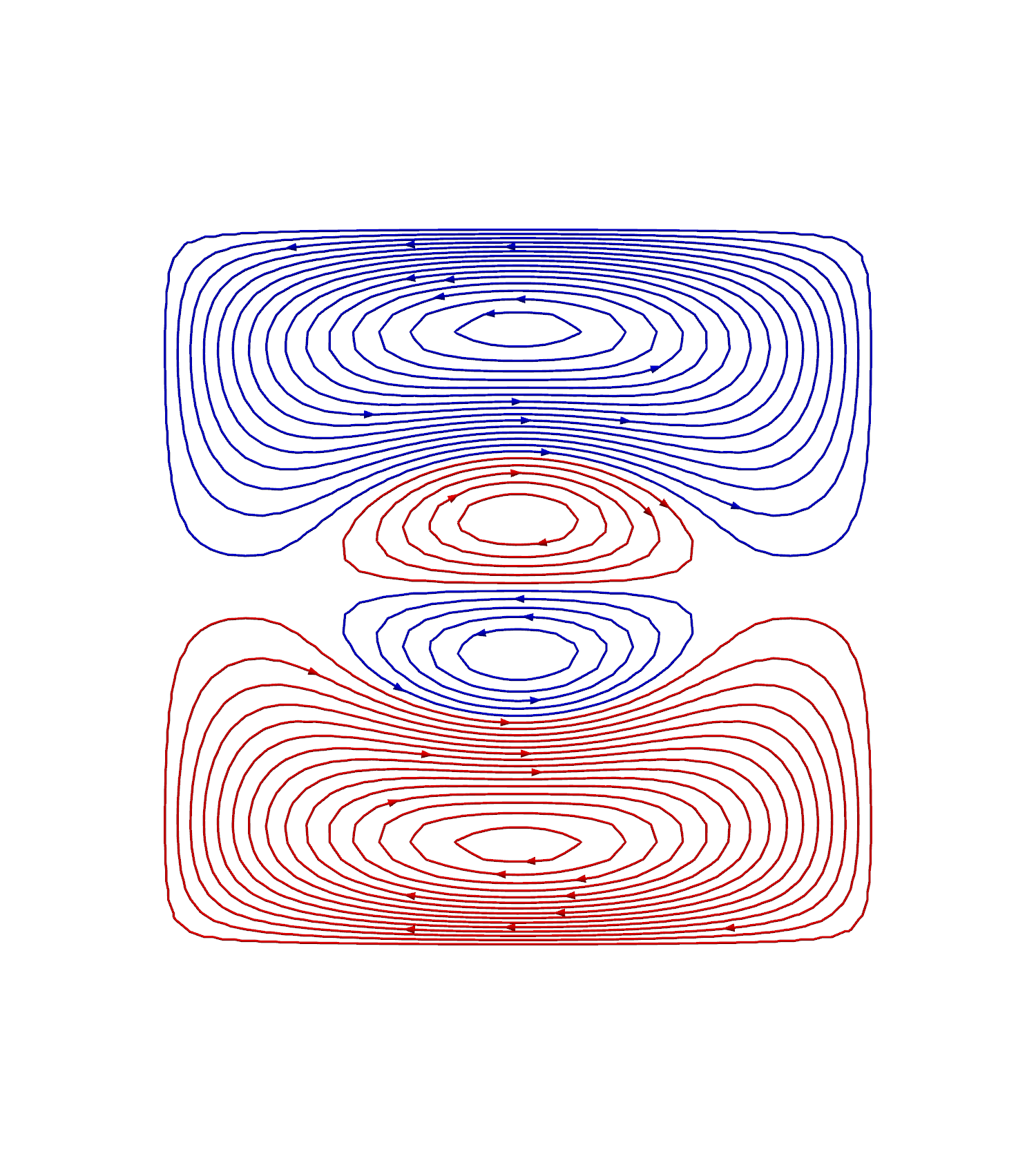
Then, we can discretize the coil into current loops. At this point, we can also specify the trace width and the copper thickness used in the PCB design.
coil.discretize(N_contours=N_contours, trace_width=trace_width, cu_oz=cu_oz)
coil.plot_coil()
Processing contour, value: -10542141.429055808
Processing contour, value: -9815097.1925692
Processing contour, value: -9088052.956082592
Processing contour, value: -8361008.719595984
Processing contour, value: -7633964.483109375
Processing contour, value: -6906920.246622768
Processing contour, value: -6179876.01013616
Processing contour, value: -5452831.773649553
Processing contour, value: -4725787.537162945
Processing contour, value: -3998743.3006763374
Processing contour, value: -3271699.0641897293
Processing contour, value: -2544654.827703121
Processing contour, value: -1817610.591216514
Processing contour, value: -1090566.3547299057
Processing contour, value: -363522.11824329756
Processing contour, value: 363522.1182433106
Processing contour, value: 1090566.354729917
Processing contour, value: 1817610.591216525
Processing contour, value: 2544654.827703133
Processing contour, value: 3271699.0641897414
Processing contour, value: 3998743.3006763496
Processing contour, value: 4725787.537162956
Processing contour, value: 5452831.773649564
Processing contour, value: 6179876.010136174
Processing contour, value: 6906920.24662278
Processing contour, value: 7633964.483109387
Processing contour, value: 8361008.719595997
Processing contour, value: 9088052.956082603
Processing contour, value: 9815097.192569213
Processing contour, value: 10542141.42905582

<pyvista.plotting.plotter.Plotter object at 0x1abb14c10>
To evaluate the effect of the shielded room, we can add it to the coil specification and it will be taken into account for estimating the magnetic field at any point
The field at some target points can be computed by doing
B_target = coil.predict(target_points)
Computing effect of shielded room
Computing magnetic field coupling matrix, 4056 vertices by 160 target points... took 0.49 seconds.
Computing scalar potential coupling matrix, 4056 vertices by 4056 target points... took 19.54 seconds.
Computing scalar potential coupling matrix, 3184 vertices by 4056 target points... took 15.88 seconds.
Done
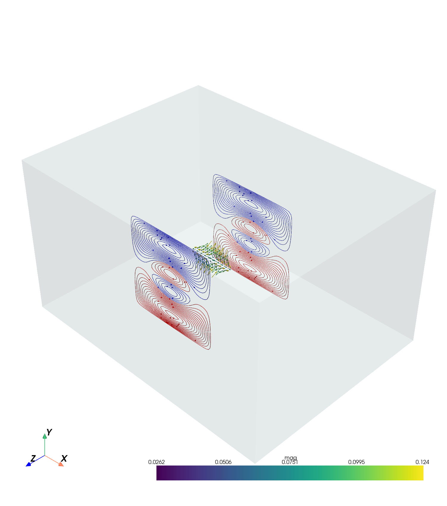
The field can be computed and plotted by doing
plotter = coil.plot_field(target_points)
Computing effect of shielded room
Computing magnetic field coupling matrix, 4056 vertices by 160 target points... took 0.54 seconds.
Computing scalar potential coupling matrix, 4056 vertices by 4056 target points... took 25.75 seconds.
Done
We can evaluate the coil for metrics such as efficiency and also compute its dimensions by doing
metrics = coil.evaluate(target_type, target_points, target_field,
                        points_z, 'all')
print(metrics)
print(f'The coil has dimensions {coil.shape} m')
Computing magnetic field coupling matrix, 3184 vertices by 8 target points... took 0.03 seconds.
Computing effect of shielded room
Computing magnetic field coupling matrix, 4056 vertices by 160 target points... took 0.53 seconds.
Computing scalar potential coupling matrix, 4056 vertices by 4056 target points... took 25.39 seconds.
Done
Computing effect of shielded room
Computing magnetic field coupling matrix, 4056 vertices by 8 target points... took 0.05 seconds.
Computing scalar potential coupling matrix, 4056 vertices by 4056 target points... took 21.82 seconds.
Done
Computing effect of shielded room
Computing magnetic field coupling matrix, 4056 vertices by 160 target points... took 0.38 seconds.
Computing scalar potential coupling matrix, 4056 vertices by 4056 target points... took 18.62 seconds.
Done
Computing effect of shielded room
Computing magnetic field coupling matrix, 4056 vertices by 160 target points... took 0.39 seconds.
Computing scalar potential coupling matrix, 4056 vertices by 4056 target points... took 16.81 seconds.
Done
Computing the inductance matrix...
Computing self-inductance matrix using rough quadrature (degree=2).              For higher accuracy, set quad_degree to 4 or more.
Estimating 34964 MiB required for 3184 by 3184 vertices...
Computing inductance matrix in 1540 chunks (458 MiB memory free),              when approx_far=True using more chunks is faster...
Computing triangle-coupling matrix
Inductance matrix computation took 18.53 seconds.
{'efficiency (nT/mA)': np.float64(7.890119425194119), 'error': np.float64(7.890119425194119), 'homogeneity (%)': np.float64(40.0), 'inductance (uH)': np.float64(4431.833804080511), 'resistance (ohm)': 7.671165403006107, 'length (m)': 156.09929599140335, 'target radius (cm)': np.float64(17.857142857142854)}
The coil has dimensions (np.float64(1.4001021891704468), np.float64(1.4166831163442335)) m
We can now interactively create paths to join the loops in the discretized coils by making “cuts”. Uncomment below to use it. coil.make_cuts()
Finally, we can export the files to KiCad
kicad_dir = Path.cwd().parent / 'hardware' / 'template' / 'headers'
pcb_dir = Path.cwd().parent / 'hardware'
if header_type[target_type] == 'vert':
    coil.save(
        pcb_fname=pcb_dir / f'{output_dir[target_type]}/first/coil_template_first.kicad_pcb',
        kicad_header_fname=kicad_dir / f'/kicad_header_{header_type[target_type]}_first_half.txt',
        bounds=(0, 750, 0, 1500), origin=(0, 750),
        bounds_wholeloop=bounds_wholeloop[target_type])

    coil.save(
        pcb_fname=pcb_dir / f'{output_dir[target_type]}/second/coil_template_second.kicad_pcb',
        kicad_header_fname=kicad_dir / f'kicad_header_{header_type[target_type]}_second_half.txt',
        bounds=(-750, 750, 0, 1500), origin=(750, 750),
        bounds_wholeloop=bounds_wholeloop[target_type])
else:
    coil.save(
        pcb_fname=pcb_dir / f'{output_dir[target_type]}/first/coil_template_first.kicad_pcb',
        kicad_header_fname=kicad_dir / f'kicad_header_{header_type[target_type]}_first_half.txt',
        bounds=(-750, 750, 0, 750), origin=(750, 0))

    coil.save(
        pcb_fname=pcb_dir / f'{output_dir[target_type]}/second/coil_template_second.kicad_pcb',
        kicad_header_fname=kicad_dir / f'kicad_header_{header_type[target_type]}_second_half.txt',
        bounds=(-750, 750, -750, 0), origin=(750, 750))
export to kicad /Users/mainak/Desktop/04_github_repos/opm_coils/hardware/Gy_coil/first/coil_template_first.kicad_pcb:

done

export to kicad /Users/mainak/Desktop/04_github_repos/opm_coils/hardware/Gy_coil/second/coil_template_second.kicad_pcb:

done
Total running time of the script: (3 minutes 18.230 seconds)