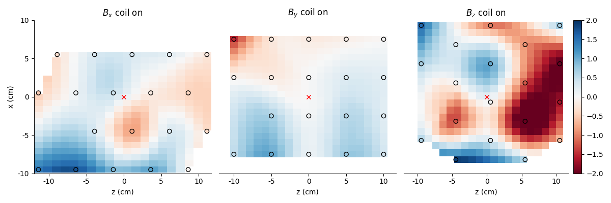
02. Planar field mapping

Example demonstrating how to map the background field along a plane.

# Authors: Mainak Jas <mjas@mgh.harvard.edu>
#          Padma Sundaram <padma@nmr.mgh.harvard.edu>

from pathlib import Path
import numpy as np

import matplotlib.pyplot as plt
from matplotlib.ticker import FormatStrFormatter
from mpl_toolkits.axes_grid1 import make_axes_locatable

from scipy.interpolate import griddata

from opmcoils.analysis import load_remnant_fields

First, we define the coordinates of the sensors from the 3D model of the sensor holders.

def get_coords(component):
    if component == 'y':

        x = [0, 5, 10, 15, 20,
             0, 5, 10, 15, 20,
                5, 10, 15, 20,
             0, 5, 10, 15, 20]

        z = [15, 15, 15, 15, 15,
             10, 10, 10, 10, 10,
                 5, 5, 5, 5,
             0, 0, 0, 0, 0]

        x = np.array(x) - 10
        z = np.array(z) - 7.5

        txt_fname = 'fine_zero_y.txt'

    if component == 'z':
        z = [17.5, 15, 17.5, 15, 17.5,
             12.5, 10, 12.5, 10, 12.5,
                   5, 7.5, 5, 7.5,
             2.5, 0, 2.5, 0, 2.5]

        x = [0, 5, 10, 15, 20,
             0, 5, 10, 15, 20,
                5, 10, 15, 20,
             0, 5, 10, 15, 20]

        x = np.array(x) - 9.5
        z = np.array(z) - 8.2

        txt_fname = 'fine_zero_z.txt'

    elif component == 'x':

        x = [2.5, 7.5, 12.5, 17.5, 22.5,
             0, 5, 10, 15, 20,
                7.5, 12.5, 17.5, 22.5,
             0, 5, 10, 15, 20]

        z = [15, 15, 15, 15, 15,
             10, 10, 10, 10, 10,
                 5, 5, 5, 5,
             0, 0, 0, 0, 0]

        x = np.array(x) - 11.4
        z = np.array(z) - 9.5

        txt_fname = 'fine_zero_x.txt'

    return x, z, txt_fname

The bias for each sensor is predefined in a dictionary.

folder = Path.cwd() / 'data'

bias = {'00:01': -0.06, '00:03': -0.74, '00:04': 0.51, '00:08': -0.43,
        '00:11': 0.11, '00:14': -0.13, '00:07': -0.42, '00:15': 1.23,
        '00:16': 0.07, '01:01': 0.42, '01:03': 0.19, '01:04': 0.02,
        '01:06': 0.22, '01:08': -0.33, '01:09': 0.30,
        '01:10': -0.12, '01:13': -1.95, '01:14': 0.65, '01:15': 0.27,
        '01:16': 0.62}

ch_names = ['01:16', '01:13', '00:04', '01:01', '01:08',
            '01:10', '01:09', '01:03', '00:16', '01:04',
                     '00:08', '00:15', '00:03', '00:11',
            '01:15', '00:01', '01:06', '00:14', '01:14']

Finally, we plot the field along the x-z plane.

fig, axes = plt.subplots(1, 3, figsize=(12, 4), sharex=True, sharey=True)
for ax, component in zip(axes, ['x', 'y', 'z']):
    x, z, txt_fname = get_coords(component)
    B = load_remnant_fields(f'{folder}/{txt_fname}',
                            ch_names=ch_names, bias=bias)

    xi = np.linspace(np.min(x), np.max(x), 20)
    zi = np.linspace(np.min(z), np.max(z), 20)
    Xi, Zi = np.meshgrid(xi, zi)

    Bi = griddata((x, z), B, (Xi, Zi), method='cubic')

    vmin, vmax = -2, 2

    im = ax.pcolormesh(Xi, Zi, Bi, vmin=vmin, vmax=vmax, cmap='RdBu')

    if component == 'z':
        divider = make_axes_locatable(ax)
        cax = divider.append_axes('right', size='5%', pad=0.1)
        cbar = fig.colorbar(im, cax=cax)

    ax.scatter(x, z, c=B, vmin=vmin, vmax=vmax,
               edgecolors='k', cmap='RdBu')
    ax.plot(0, 0, 'rx')

    ax.xaxis.set_major_formatter(FormatStrFormatter('%d'))
    ax.yaxis.set_major_formatter(FormatStrFormatter('%d'))
    ax.spines['right'].set_visible(False)
    ax.spines['top'].set_visible(False)

    ax.set_yticks(np.linspace(-10, 10, 5))
    if component != 'x':
        ax.spines['left'].set_visible(False)
        ax.tick_params(axis='y', which='both', left=False)

    ax.set_xticks(np.linspace(-10, 10, 5))
    ax.set_xlabel('z (cm)')
    ax.set_title(f'$B_{component}$ coil on')

axes[0].set_ylabel('x (cm)')
plt.tight_layout()
plt.show()